Regional smoothing using R
Recently, we published a project examining the geographic spread of movie preferences, inspired by the New York Times’ map of American television tastes and Jack Grieve’s research on the spread of new words.
Since figuring how to do this can be a somewhat time-consuming process (h/t Jack Grieve for his help here), I decided to put together a step-by-step tutorial on how to smooth data. This guide is in R, but doesn't require much R knowledge.
Smoothing: A word of warning
Smoothing is generally used to identify hot spots, or areas that have a high likelihood of differing from neighboring locations on attributes like births, crime, or disease. Through statistical means, this technique removes some of the variance you'd normally see in a choropleth, and helps give a bird's eye overview to a set of results. Unless your aim is to help provide a summary snapshot of granular data, smoothing may not be necessary, or even desired.
What we’ll learn (technical version)
Regional smoothing in R involves the use of Roger Bivand’s Spatial Dependence package to create neighbors lists through the nb2listw() function, and using this list to compute the Gettis-Ord statistic/local G statistic/z-score.
What we’ll learn (human version)
All these fancy words mean that for every single geographic location in your dataset, we’ll be calculating a list of neighboring locations. Based on the values of these neighbors, we’re going to calculate the probability that each location in question has a high value.
What you’ll need: Dependencies
Before we jump into R, we’ll have to set up a few dependencies. I’ve put together a list of these, with instructions available in each link:
What you’ll need: Data
A shapefile which corresponds to the geographic boundaries you’re looking to map, which contains a data set of values which correspond to the geographies you’re mapping.
If you’ve got data and a shapefile but don’t know how to combine them into a single file, here are a couple of great guides to doing so.
If you don’t have a dataset in mind and just want to get a hang of smoothing, you can download the shapefile I’ve used for this guide. I’ve created it using:
- A county-level shapefile
- A county-level data set of the percentage of U.S. adults who only have a high school diploma (2011-2015)
What does this data look like when we map it?
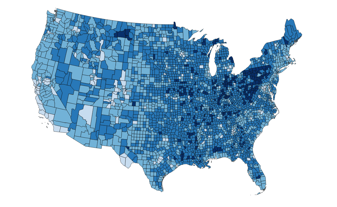
There are some pretty clear trends here, but let's use smoothing to make these stand out a little more.
Code time
In the original paper that J. K. Ord and Arthur Getis published some 20 years ago, the pair suggested a measure called the Getis-Ord Gi* to statistically test for geographical hot spots (e.g., of disease, crime, etc.). This is the method we'll be using, and employs what is commonly referred to as the Getis-Ord local statistic (if you’re interested in reading more, I’d suggest ESRI’s quick guide, or the original academic paper).
First, we’ll have to load up a few packages (if you see an error about proj_defs.dat, this link should help):
library(proj4)
library(spdep)
library(maptools)
library(rgdal)
Next, read the shapefile into R as a Large Spatial Polygon Data Frame:
shapefile <-readShapePoly("/directory/shapefile.shp")Set the projection for this shapefile, since R doesn’t read it otherwise. Below, I’m using the code EPSG:4326 (a list of these codes can be found here), which refers to the same projection that's commonly used by the U.S. Dept. of Defense:
proj4string(shapefile)<-CRS("+proj=longlat +init=epsg:4326")If you’d like to change the projection (I like the Albers projection when looking exclusively at the U.S.), you can do so with another line of code:
shapefile_albers <-spTransform(shapefile, CRS("+init=ESRI:102003"))Next, let's convert the shapefile into a regular data frame and substitute any missing values with 0 (you won't need this second line if you don't have any missing values associated with your locations).
shapefile_df <- as(shapefile_albers, "data.frame")
shapefile_df[is.na(shapefile_df)] <-0
Now we can start setting out the neighbors list. Neighbors of a location can usually be defined in one of three ways:
- As polygons that share a border with the location in question
- As being within a certain distance from the location in question
- As a specific number of neighbors that are closest to the location; the precise number of neighbors us up to us. This is calculated using the k-nearest neighbors (KNN) algorithm.
In this tutorial I'll focus on the KNN method, but if you'd like to explore the first two, I'd recommend this excellent powerpoint presentation by Elisabeth Root.
K-Nearest neighbors are calculated using coordinates, so we need to specify the coordinate system to be used for our shapefile, as well as the list of counties that we'll be calculating neighbors for.
coords <- coordinates(shapefile_albers)
IDs<-row.names(as(shapefile_albers, "data.frame"))
The number of neighbors you use is going to significantly affect the degree of smoothing, so I'd suggest using your best judgment and experimenting with a range. Let's set up the neighbors list using the 50 nearest neighbors for each location; this is high, but is useful for the sake of illustration. To make sure that we don’t get weird doughnut-type holes around each high-value area, we'll need to make sure that each area is included (somewhat paradoxically) in its list of neighbors.
knn50 <- knn2nb(knearneigh(coords, k = 50), row.names = IDs)
knn50 <- include.self(knn50)
We’re now ready to create the localG statistics — these represent the likelihood that each location has a high percentage of adults with a high school-only education. We’ll first create a regular data frame, ensure that its NA values are replaced by 0s, and calculate localGs for each of the columns which contain our data. Finally, we'll write the data frame to a CSV.
# Creating the localG statistic for each of counties, with a k-nearest neighbor value of 5, and round this to 3 decimal places
localGvalues <- localG(x = as.numeric(shapefile_df$hs_pct), listw = nb2listw(knn50, style = "B"), zero.policy = TRUE)
localGvalues <- round(localGvalues,3)

# Create a new data frame that only includes the county fips codes and the G scores
new_df <- data.frame(shapefile_df$GEOID)
new_df$values <- localGvalues

#Huzzah! We are now ready to export this CSV, and visualize away!
write.table(row.names = FALSE,new_df, file = "smooooothstuff.csv", sep=",")
The end result:
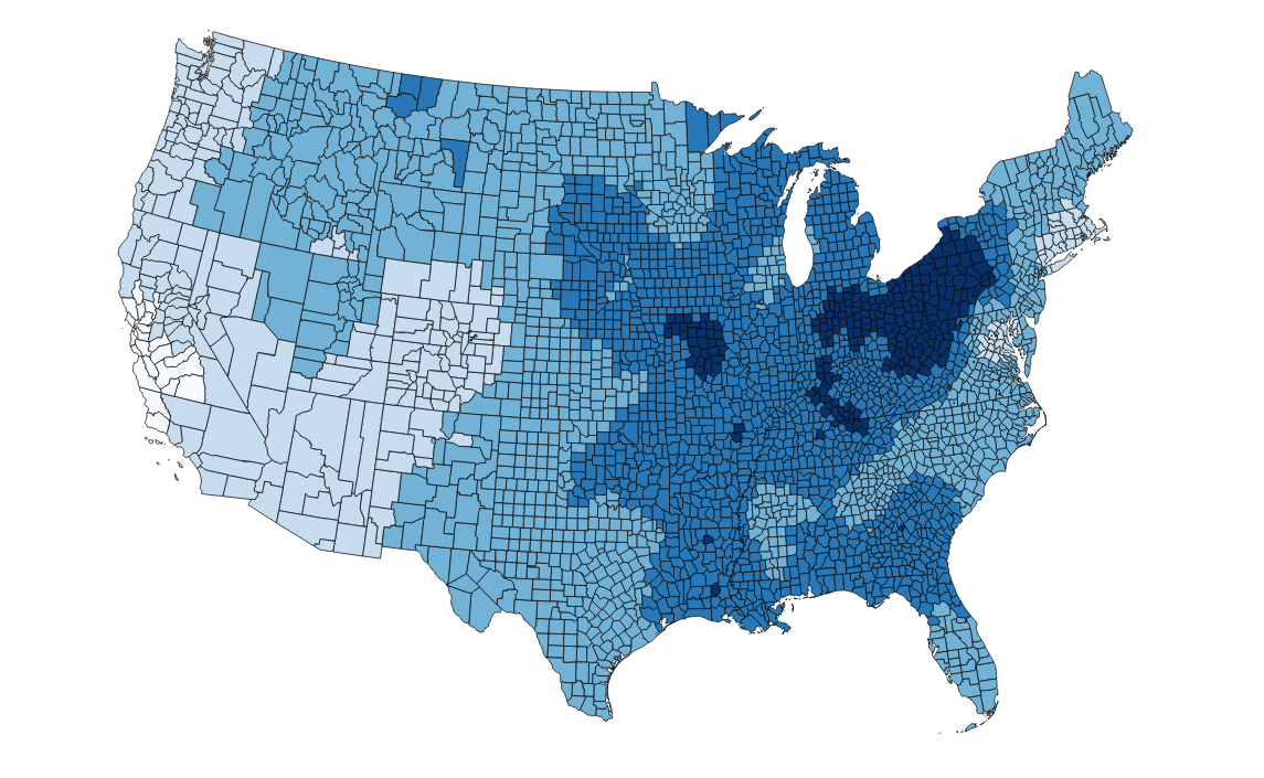
Here's the complete script! Hey map, are you a classic Rob Thomas ft. Santana track? Because you're v. smooth.
Additional Resources
- There’s a great tutorial by Elisabeth Root, of UC Colorado's Dept. of Geography, which explains the differences between the various neighbors weights algorithms. This is terrific and somewhat more stats-heavy, but I found it to be a very clear guide.
- For any in-depth questions, here's message board for R and geospatial work.
- Spatial Regression Analysis in R: A Workbook
- Creating neighbors (Roger Bivand’s book chapter)